
Our daily lives are inundated with predictions about the future, but they usually suck. Most of us know to be skeptical when we encounter election forecasts on cable news or stock picks at the Thanksgiving table. They’re terrible because human brains are ill-equipped to grasp uncertainty, and casual pundits typically neglect to back their predictions with logic or evidence.
Intelligence agencies, however, must approach predictions in a more careful and systematic manner. After all, when a country’s national security or geopolitical standing is at stake, the cost of failure can be catastrophic.
Declassified reports on the CIA’s website show that analysts at the agency had experimented with tools from Bayesian statistics to make high-stakes predictions. In this article, we’ll look at how the CIA applied Bayes’ theorem to study and forecast geopolitical events.
What is a Probability?
First, let’s briefly discuss how Bayesian statistics differs from the “traditional” statistics that you learn in a Statistics 101 class. It stems from a philosophical difference in the definition of a “probability”.
“Traditional” statistics that you were likely taught is based on a “frequentist” interpretation of probability. In this paradigm, a probability is defined as the proportion of times that a given outcome occurs when a random event is repeated infinite times. A typical example involves repeatedly flipping a fair coin. As the number of coin flips becomes progressively larger, the proportion of heads gradually approaches 50%. So the probability of flipping heads is 0.5.
The Bayesian paradigm defines a probability as a degree of belief. This corresponds to how we think about probability in everyday life, such as when we say something like: “I believe the senator has a 25% chance of getting reelected.” When probabilities represent degrees of belief, we have a way to account for uncertainty in our logical reasoning about whether something is “True” or “False”.
Bayes’ Theorem
The fundamental axiom of Bayesian analysis is Bayes’ theorem:
\[P(belief \;|\; data) = \frac{P(data \;|\; belief) \times P(belief)}{P(data)}\]Where:
-
P(belief) is our prior probability. This probability represents the beliefs that we bring to the table before seeing any new data. In other words, this is your starting hypothesis.
-
P(data | belief) is the likelihood. This probability represents how likely you are to see your data if your starting hypothesis is true.
-
P(belief | data) is the posterior probability. This is the probability that your belief is true given the data that you’ve seen.
(In the equation above, dividing by P(data) ensures that our posterior probability is a value between 0 and 1.)
Bayes’ theorem is a statistical identity that allows us to carefully manage what we know and what we observe to make careful and consistent predictions. A close look at the equation above will reveal how Bayes’ theorem can serve as a powerful analytical tool.
First, it allows us to make conversions between:
- P(belief | data): The probability that your belief is true, given observed data.
- P(data | belief): The probability you’d see the observed data, if your belief is true.
Pay close attention, because the probability of A given B and the probability of B given A are not the same. In fact, confusing the two can be a path to Fox News-style stupidity and bigotry. In his book The Black Swan, Nassim Nicholas Taleb observes that:
“Many people confuse the statement ‘almost all terrorists are Moslems’ with ‘almost all Moslems are terrorists.’ Assume that the first statement is true, that 99 percent of terrorists are Moslems. This would mean that only about .001 percent of Moslems are terrorists, since there are more than one billion Moslems and only, say ten thousand terrorists, one in a hundred thousand. So the logical mistake makes you (unconsciously) overestimate the odds of a randomly drawn individual Moslem person (between the age of, say, fifteen and fifty) being a terrorist by close to fifty thousand times!”
Second, Bayes’ theorem provides a framework for us to iteratively update our beliefs as we observe new data over time. Our prior probability is our starting hypothesis. We factor in the likelihood of seeing the new data if our starting hypothesis is true. We revise our beliefs given the data that we observe. Rinse and repeat.
Now that we’re equipped with a basic familiarity of Bayes’ theorem, let’s take a look at some ways that it was applied at the CIA.
Example #1: A Conflict in the Middle East
The paper “Bayesian Analysis for Intelligence: Some Focus on the Middle East”, published in the CIA journal Studies in Intelligence, contains a guided example on how Bayes’ theorem can be used to forecast a conflict in the Middle East.
According to the paper, suppose that we have two competing hypotheses:
H1: Israel is planning a major offensive against Syria within 30 days.
H2: Israel is not planning such an offensive.
Furthermore, suppose that a CIA analyst believes that there’s a 10% chance that Israel will launch the offensive:
\[P(H_1) = 0.1\] \[P(H_2) = 0.9\]After the analyst has made these predictions, the following news rolls in:
“Israeli Finance Minister Rabinowitz stated that the nation’s economic situation is one of war and scarcity, not one of peace and prosperity.” (Jerusalem Radio, 20 February, unclassified)
We will refer to this piece of news by the variable E (for “event”).
The analyst believes that the probability that the Finance Minister would say this if Israel is planning an offensive to be 99%, and the probability that he’d say this if Israel is not planning an offensive is 88%. So:
\[P(E \;|\; H_1) = 0.99\] \[P(E \;|\; H_2) = 0.8\]We can now plug these numbers into Bayes’ theorem. To calculate the posterior probability of the first hypothesis, take the formula…
\[P(H_1 \;|\; E) = \frac{P(E \;|\; H_1) \times P(H_1)}{P(E)}\]… and plug in what we know:
\[P(H_1 \;|\; E) = \frac{0.99 \times 0.1}{P(E)}\]The formula above is still missing P(E): the probability of the Israeli Finance Minister’s statement, regardless of the analyst’s prior beliefs. We actually have enough information to calculate this with the help of some probability rules:
\[P(E) = P(E \;and\; H_1) + P(E \;and\; H_2)\]which can be expanded to:
\[P(E) = P(E \;|\; H_1) \times P(H_1) + P(E \;|\; H_2) \times P(H_2)\]We can now solve for P(E):
\[P(E) = 0.99 \times 0.1 + 0.8 \times 0.9 = 0.819\]Plugging all of our numbers back into Bayes’ theorem gives us the posterior (revised) probability of whether Israel will launch an offensive in light of the Finance Minister’s statement.
\[P(H_1 \;|\; E) = \frac{P(E \;|\; H_1) \times P(H_1)}{P(E)} = \frac{0.99 \times 0.1}{0.819} = 0.12\]We can do the same for the posterior probability that Israel will not launch an offensive:
\[P(H_2 \;|\; E) = \frac{P(E \;|\; H_2) \times P(H_2)}{P(E)} = \frac{0.8 \times 0.9}{0.819} = 0.88\]So given knowledge of Finance Minister Rabinowitz’s statement, the CIA analyst should update the probability of an Israeli offensive to 0.12, and the probability of no offensive to 0.88.
Example #2: Chinese Intervention in the Korean War
The Korean War took place from 1950 to 1953, beginning with the North Korean military crossing the 38th parallel and entering South Korean territory. The United States joined the war in support of South Korea. Under the leadership of General Douglas MacArthur, U.S. and South Korean forces took the fight into North Korean territory, pushing as far as the Yalu River. This prompted China’s People’s Liberation Army to intervene in late-1950 on behalf of North Korea, which ultimately led to a military stalemate.
Since the PLA’s intervention was a turning point in the Korean War, the CIA conducted a retrospective simulation to see if Bayesian analysis could have predicted Chinese intervention in 1950. The results are detailed in a 1968 intelligence report titled “Bayes’ Theorem in the Korean War”.
The simulation involves three competing hypotheses that an intelligence analyst in 1950 would have needed to evaluate:
H1: PLA troops will cross the Yalu River in large numbers (more than 100,000) to engage in full combat on the side of the North Koreans.
H2: China will intervene but not with large numbers of combat troops.
H3: China will not intervene with its own combat troops in the Korean War.
The simulation begins with a CIA analyst’s likely assessment on September 15, 1950. An analyst on this day would likely have known that:
-
“[Beijing] is clearly concerned about the potential threat of its security from the gathering US military strength in South Korea.”
-
“Consolidation of domestic control and final defeat of Chiang Kai-shek, however, rate higher in the Chinese Communist scale of priorities than the expansion of Communism on the Korean peninsula.”
Using a mapping between language found in contemporaneous intelligence reports and numerical probabilities:
| Verbal Form | Numerical Equivalent |
|---|---|
| Certainly, sure to, no question about | 1.0 |
| Almost certainly | 0.9 |
| Very probably | 0.8 |
| Probably | 0.7 |
| On balance, somewhat more likely than not | 0.6 |
| Like as not, even money | 0.5 |
| Somewhat less than even chance | 0.4 |
| Probably not | 0.3 |
| Very probably not | 0.2 |
| Almost certainly not | 0.1 |
| Certainly not, impossible | 0.0 |
The report suggests that our hypothetical analyst would have assigned the following priors based on what’s known about the People’s Republic of China on September 15.
\[P(H_1) = 0.1\] \[P(H_2) = 0.3\] \[P(H_3) = 0.6\]Discussion about subsequent news that the analyst would have received is highly redacted. Nevertheless, we know that each piece of news in the unredacted report would have been accompanied by likelihoods of the news occurring if the hypotheses above were true. This would have allowed for successive rounds of belief updates using Bayes’ theorem, as shown in the following graph:
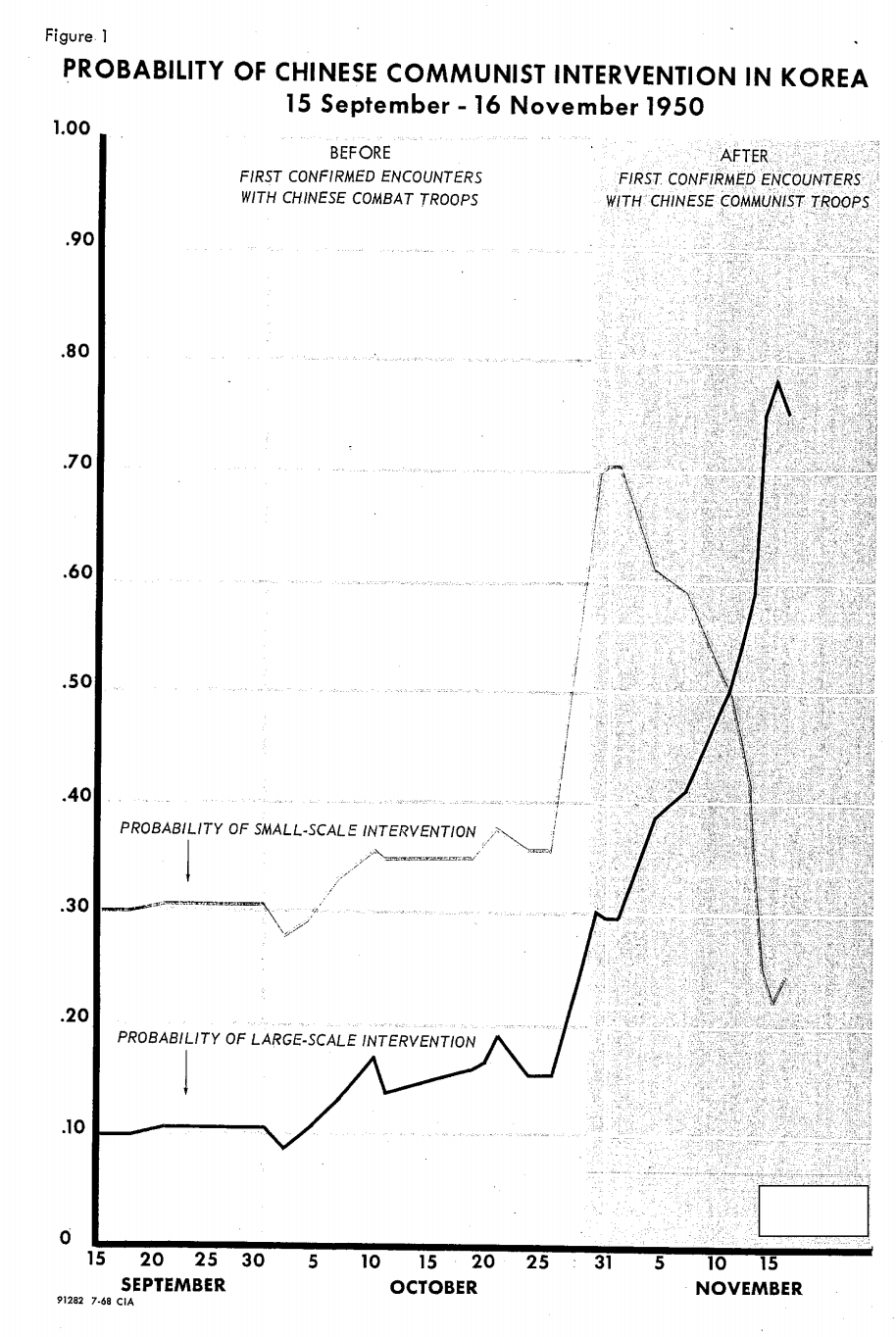
The report concludes that, by mid-November of 1950, the analyst would have found the probability of H1 – a large-scale Chinese intervention in the war – to be 0.75. This is an enormous change from the mid-September probability of 0.1.
Additional Resources
For a fun and painless introduction to Bayesian statistics, I highly recommend Will Kurt’s Bayesian Statistics the Fun Way. More information about how the CIA used Bayesian techniques can be found in the 1975 study “Handbook of Bayesian Analysis for Intelligence”.
Header photo by Juli Kosolapova on Unsplash